Accelerating materials research with Duke Compute Cluster’s (DCC) NVIDIA Tesla P100 GPUs

Leveraging DCC’s NVIDIA Tesla P100 GPUs, in this post I demonstrate how GPU acceleration within FHI‑aims and ELPA can speed up all-electron DFT calculations by a factor of ~2x on systems exceeding 3,000 atoms and 50,000 basis functions.

Firstly, May the 4th be with you!

As mentioned in an earlier post, this semester I had the privilege of setting up and optimizing the Density Functional Theory (DFT)¹ code FHI-aims² on the Duke Compute Cluster (DCC) for students in the ME511 (Computational Materials Science) course as well as for lab members of the AIMS Group to perform materials simulations for research and education. As part of this endeavor, I explored how utilizing GPUs can accelerate electronic structure calculations. I have documented my efforts to configure this setup here.

GPU implementation

Kohn-Sham DFT (KS-DFT) is considered to be the primary tool for computational materials research in a wide range of areas in science and engineering. FHI-aims is an all-electron electronic structure code based on numeric atom-centered orbitals that solves the Kohn-Sham eigenvalue problem,

\[\hat{h}^{\mathrm{KS}}\left|\psi_l\right\rangle=\epsilon_l\left|\psi_l\right\rangle\]

where, $\ket{\psi_l}$ are effective single-particle orbitals (KS orbitals) with the Hamiltonian $\hat{h}^{\mathrm{KS}}$ in its scalar-relativistic form,

\[\hat{h}_{KS}=\hat{t}_s+\hat{v}_{ext}+\hat{v}_H[n]+\hat{v}_{xc}[n].\]

Here, $\hat{t}_s$ is the kinetic‑energy operator, $\hat{v}_{ext}$ is the external potential, $\hat{v}_H[n]$ is the Hartree potential of the electrons, and $\hat{v}_{xc}[n]$ is the exchange-correlation potential. The density $n$ that minimizes the total energy is obtained through a self‑consistent field (SCF) cycle.

Recent improvements in the code have made it possible to utilize GPUs to accelerate segments of this process. Readers are referred to W.P. Huhn, B. Lange, V.W.-z. Yu et al./Comput. Phys. Commun. 254 (2020) 107314³ and V.W.-z. Yu, J. Moussa, P. Kůs et al./Comput. Phys. Commun. 262 (2021) 107808⁴ for a deeper dive into the implementation.

GPU support in FHI-aims is focused on two computational hotspots that dominate a semi-local DFT self-consistent field (SCF) cycle.

1. Real-space operations

These calculations include Hamiltonian and overlap matrix integration, electron density update, forces and stress tensor calculation which scale linearly as $O(N)$ with system size, N. A real-space domain decomposition (RSDD) algorithm splits the integration grid into compact “batches” so that the Hamiltonian can be reformulated as,

\[h_{i j}^{u c}=\sum_v h_{i j}^{u c}\left[B_v\right]\]

where,

\[h_{i j}^{u c}\left[B_\nu\right]=\sum_{\boldsymbol{r} \in B_\nu} w(\boldsymbol{r}) \varphi_i^*(\boldsymbol{r}) \hat{h}_{K S} \varphi_j(\boldsymbol{r})\]

is the contribution of batch $B_\nu$ to the real-space Hamiltonian matrix element $h_{i j}^{u c}$. Each batch becomes a small dense matrix that is offloaded to the GPU as cuBLAS function calls. A large number of such batches stream through in parallel while keeping the CPU-GPU communication minimal by holding batches on-device until calculations are finished. An analogous method is used for the density matrix $n_{ij}[B_\nu]$ and force calculations.

2. Kohn-Sham eigensolver (ELPA)

This segment scales as $O(N^3)$ and is considered to be the workhorse of DFT. This step focuses on solving the generalized eigenproblem in its matrix form,

\[H C=S C \Sigma\]

where, H is the Hamiltonian, S is the overlap, C is the eigen vector, and $\Sigma$ is the eigenvalue matrix of the system. FHI-aims delegates this step to the ELPA⁵ eigensolver through the ELSI interface, whose ELPA2 two-stage tridiagonlization replaces local BLAS calls with their cuBLAS equivalent and adds a CUDA kernel for the computationally complex Householder back-transformation step to an eigenvector $\boldsymbol{x}$,

\[\left(\boldsymbol{I}-\tau \boldsymbol{v} \boldsymbol{v}^*\right) \boldsymbol{x}=\boldsymbol{x}-\tau \boldsymbol{v}\left(\boldsymbol{v}^* \boldsymbol{x}\right) .\]

This process is depicted in Fig. 1.

Figure 1: The computational steps of the two-stage tridiagonlization algorithm implemented in ELPA. Ref. [V.W.-z. Yu, J. Moussa, P. Kůs et al.]

Similar to the GPU offloaded real-space operations discussed earlier, data stay resident on the GPU between stages to minimize communication latency.

Benchmark systems and platform

To demonstrate the GPU acceleration in the code, I ran benchmark tests on the following two materials systems,

(1). 3,000 atom Cu$_2$BaSnS$_4$ semiconductor (CBTS) supercell with 80,250 basis functions
(2). 3,376 atom Graphene-covered SiC surface model with 51,576 basis functions

Their crystal structures are shown in Fig. 2.

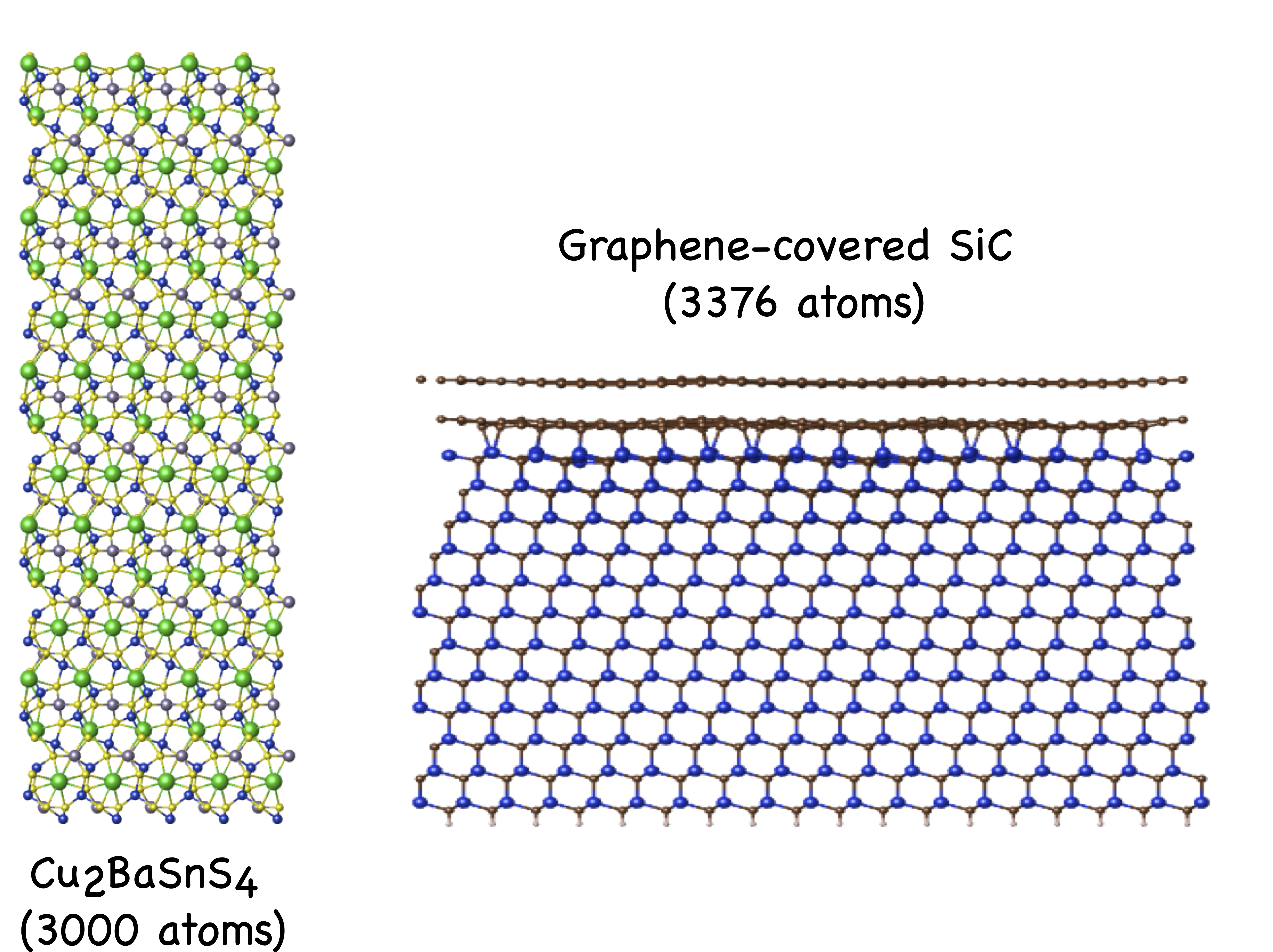Figure 2: The crystal structures of Cu$_2$BaSnS$_4$ (left) and Graphene-covered SiC (right).

These benchmarks were performed on DCC’s courses-gpu nodes. Each of these nodes consist of 44 $\times$ Intel(R) Xeon(R) CPU E5-2699 v4 physical cores (88 hyperthreads) operating at a nominal frequency of 2.2 GHz and 479 GB of RAM. However, one core is reserved for the virtualization hypervisor (VMWare ESXi) and another for the guest OS, making 42 physical cores (84 hyperthreads) available for calculations. The nodes are networked through Mellanox ConnectX-4 Infiniband connections. Additionally, each node is equipped with 2 $\times$ NVIDIA Tesla P100 GPUs with 16 GB RAM.

nvidia-smi provides the following information on a typical courses-gpu node.

(py3) ukh at dcc-courses-gpu-07 in ~
$ nvidia-smi
Fri Apr 25 22:29:34 2025
+-----------------------------------------------------------------------------------------+
| NVIDIA-SMI 560.35.05              Driver Version: 560.35.05      CUDA Version: 12.6     |
|-----------------------------------------+------------------------+----------------------+
| GPU  Name                 Persistence-M | Bus-Id          Disp.A | Volatile Uncorr. ECC |
| Fan  Temp   Perf          Pwr:Usage/Cap |           Memory-Usage | GPU-Util  Compute M. |
|                                         |                        |               MIG M. |
|=========================================+========================+======================|
|   0  Tesla P100-PCIE-16GB           On  |   00000000:13:00.0 Off |                    0 |
| N/A   21C    P0             24W /  250W |       0MiB /  16384MiB |      0%      Default |
|                                         |                        |                  N/A |
+-----------------------------------------+------------------------+----------------------+
|   1  Tesla P100-PCIE-16GB           On  |   00000000:1B:00.0 Off |                    0 |
| N/A   21C    P0             24W /  250W |       0MiB /  16384MiB |      0%      Default |
|                                         |                        |                  N/A |
+-----------------------------------------+------------------------+----------------------+

+-----------------------------------------------------------------------------------------+
| Processes:                                                                              |
|  GPU   GI   CI        PID   Type   Process name                              GPU Memory |
|        ID   ID                                                               Usage      |
|=========================================================================================|
|  No running processes found                                                             |
+-----------------------------------------------------------------------------------------+

These calculations were performed with FHI-aims v250403 built with Intel oneAPI LLVM Fortran, C, C++ compilers v2025.0.4, Intel MPI v2021.14, Intel MKL v2025.0, and CUDA v12.4. The default ELPA eigensolver (v2020.05.001) that comes bundled with FHI-aims was used as the eigensolver.

Benchmark results

For the 3,000 atom Cu$_2$BaSnS$_4$ structure with 80,250 basis functions, the calculation run on two nodes halted with the following error message, due to insufficient GPU memory.

/hpc/home/ukh/local/FHIaims/FHIaims-intel-gpu/external_libraries/elsi_interface/external/ELPA/ELPA-2020.05.001/src/cudaFunctions.cu:90
Error in cudaMalloc: out of memory

Since a single node only provides 16 GB of GPU RAM per device, increasing the node count resolved this issue. The results of the benchmark tests are shown in Fig. 3.

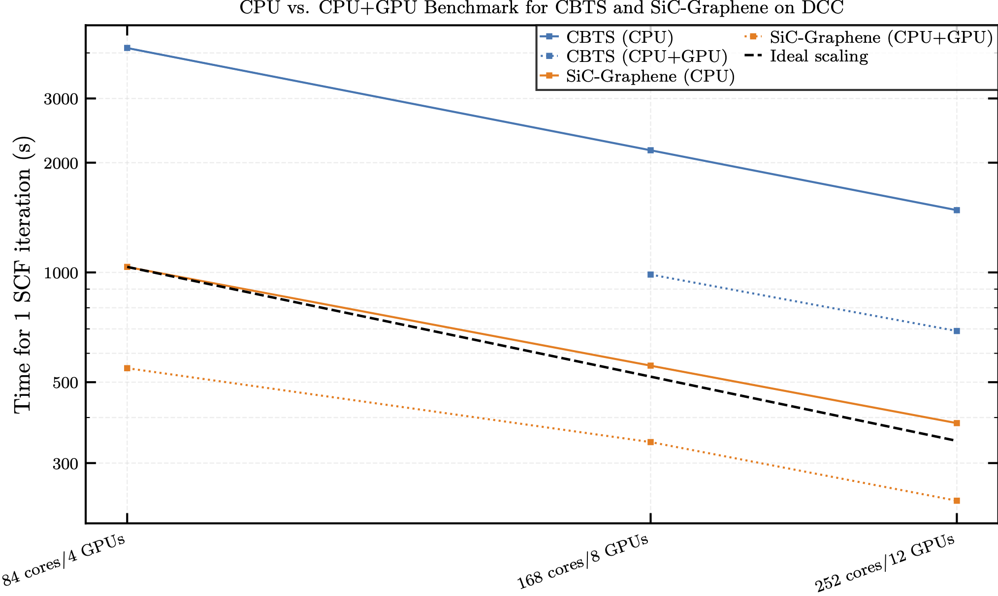Figure 3: The benchmark results for CBTS (blue) and SiC-covered Graphene (orange) calculated with FHI-aims comparing timing for a single SCF iteration with and without GPU acceleration. Solid lines represent CPU only runs and dotted lines represent runs with GPU acceleration enabled. The dotted black line represents ideal scaling.

As an example, the break down of several key timing steps for a single SCF iteration for the 252 core/12 GPU CBTS run is given in Table 1.

Table 1: Timing of key stages in a single SCF iteration with and without GPU acceleration for the 252 core/12 GPU CBTS run

Step	CPU (s)	CPU+GPU (s)
Real-space Hamiltonian integration	31.07	26.75
Charge density update	106.85	54.767
Kohn-Sham equation solution (eigensolver)	1331.15	596.42

Table 1 shows the different calculation steps that were accelerated with GPUs in comparison to their CPU-only counterparts. For this case, the most significant speedup (~2.2x) is due to the eigensolver, which is expected since this is essentially the workhorse of DFT.

Looking at the outcomes in Fig. 3, we observe an average ~2× acceleration for CBTS and ~1.7× for SiC‑Graphene, measured per SCF iteration at equal core/GPU counts. This is already a significant improvement in speedup considering these large system sizes and may be improved further by,

• Building FHI-aims with a more recent version of the ELPA eigensolver that features more modern and efficient GPU optimizations.

• Experimenting with different Scalapack matrix block sizes by adjusting the scalapack_block_size <block_size> parameter and changing the points_in_batch <value> value that targets the number of integration points per batch offloaded to the GPU.

• Enabling the NVIDIA Multi-Process Service (MPS) allows work from different MPI processes to be executed concurrently on the GPU, so that memory transfer and computation requests from different MPI processes are automatically overlapped whenever possible. This typically increases the overall GPU utilization.

In summary, the NVIDIA Tesla P100 GPUs on DCC do a great job accelerating calculations for materials simulations, especially for large scale systems. I gratefully acknowledge the Duke Research Computing Team for providing access to DCC and for the insightful discussions that helped shape this work. Feel free to leave any feedback in the comments and please reach out if you need any help setting up your calculations with GPU acceleration.

References

1. P. Hohenberg and W. Kohn, Inhomogeneous Electron Gas, Phys. Rev. 136, B864 (1964). DOI: https://doi.org/10.1103/PhysRev.136.B864 ↩

2. V. Blum, R. Gehrke, F. Hanke, P. Havu, V. Havu, X. Ren, K. Reuter, and M. Scheffler, Ab initio molecular simulations with numeric atom-centered orbitals, Computer Physics Communications 180, 2175 (2009). DOI: https://doi.org/10.1016/j.cpc.2009.06.022 ↩

3. W. P. Huhn, B. Lange, V. W. Yu, M. Yoon, and V. Blum, GPU acceleration of all-electron electronic structure theory using localized numeric atom-centered basis functions, Computer Physics Communications 254, 107314 (2020). DOI: https://doi.org/10.1016/j.cpc.2020.107314 ↩

4. V. W. Yu, J. Moussa, P. Kůs, A. Marek, P. Messmer, M. Yoon, H. Lederer, and V. Blum, GPU-acceleration of the ELPA2 distributed eigensolver for dense symmetric and hermitian eigenproblems, Computer Physics Communications 262, 107808 (2021). DOI: https://doi.org/10.1016/j.cpc.2020.107808 ↩

5. Hans-Joachim Bungartz et. al.: ELPA: A Parallel Solver for the Generalized Eigenvalue Problem, Advances in Parallel Computing, Vol. 36 Parallel Computing: Technology Trends, DOI: 10.3233/APC200095 Online version: https://ebooks.iospress.nl/doi/10.3233/APC200095 ↩

Sign up to get updates on my latest blog posts!

Thank you!

You have successfully joined my subscriber list.