Error estimation in band structures

Accurate error estimation is highly beneficial for quantifying differences in band structures of materials. This post explores utilizing the root-mean-square error (RMSE) for comparing band structures calculated with the FHI-aims code. This method can help us quickly gauge the agreement between two band structures and guide more informed decisions in materials simulations.

The band structure of a material describes the range of energy levels that electrons are allowed to occupy. It encodes crucial information about a material’s electrical conductivity and forms the basis for predicting various electronic and optical properties including band gap values, excitations, and conduction mechanisms providing deeper insights in semiconductor and photovoltaics applications¹.

While calculating band structures is standard practice in materials science helping us visually gauge the similarities and differences between electronic structure methods, it is often useful to quantify these comparisons beyond observables such as band gaps. For example, quantifying the difference between band structures calculated with the GW approximation² vs. HSE06 hybrid functionals³, different basis set tiers such as intermediate vs. tight, or identifying the effects of spin-orbit coupling (SOC) onto a band structure.

For this purpose, I extended the aimsplot_compare.py tool within FHI-aims/utilities to use the root-mean-square error (RMSE) which measures the average difference between two statistical datasets- in our case, two band structures. Mathematically, it is the standard deviation of the residuals which represent the distance between the regression line and the data points⁴. In simple terms, RMSE can be formulated as shown below.

\[RMSE=\sqrt{\sum_{i=1}^n \frac{\left(\hat{y}_i-y_i\right)^2}{n}}\]

where, $\hat{y}_i$ is the predicted value, $y_i$ is the observed value, and $n$ is the number of data points. Let’s see how we can use this to create a model to compare two band structures.

RMSE algorithm for comparing band structures

The discussion here should be applicable to any first-principles electronic structure code (e.g., VASP, Abinit, Siesta, Quantum Espresso, Elk), however, the code I present in this post is targeted for FHI-aims⁵.

To compute an RMSE for band structures, we need,

1. Corresponding k-points: Make sure the two band structures in question have the same k-path segmentation, number of k-points per segment, and same order of k-path segments.

2. Same reference: Typically, we want both sets of energies aligned to the same reference, often the Fermi level or some valence-band maximum (VBM). This code shifts band energies set by a user-supplied offset if needed.

3. Common energy window: It is important to find a one-to-one mapping of bands between the band structures. In some cases a deep core state band with -1000 eV may be matched erroneously with a band that is just -20 eV leading to a high RMSE value. This is remedied by selecting a common set of bands for comparison within a selected energy window. If the user does not provide an energy window, the code selects a default range.

Provided these conditions, the code then filters out all the bands that lie entirely outside the chosen energy window. Then, it matches the columns up to the minimum number of bands present in both datasets within that window. Next, it computes the squared difference at each k-point for those matched bands. Finally, it takes the mean and the square root, providing the root-mean-square (RMSE) value. It also outputs a plot of the band structure comparison.

Mathematically, for a given energy window,

\[RMSE=\sqrt{\frac{1}{N} \sum_{k=1}^{N_k} \sum_{i=1}^{n_{bands}}\left(E_2(k, i)-E_1(k, i)\right)^2}\]

where, $N = N_k \times n_{bands}$ is summed over all band segments.

Code and usage

The code snippet below demonstrates the main functionality of the process, where we read two sets of band information, align and filter them by an energy window, and then compute the RMSE. It currently does not support colinear spin calculations, but I intend to incorporate that in the future. The code also accounts for the degeneracy of bands when SOC is enabled.

##############################
# 6) Compute RMSE if nPlots=2
##############################
def filter_bands_by_energy_range(E, y_min, y_max):
    # E shape: (nK, nB)
    keep = []
    nK, nB = E.shape
    for b in range(nB):
        arr = E[:, b]
        if arr.max() < y_min or arr.min() > y_max:
            continue
        keep.append(b)
    if len(keep) > 0:
        return E[:, keep]
    else:
        return np.zeros((nK, 0))


if nPlots == 2:
    sum_sq = 0.0
    nvals = 0

    # Do a naive pass over band_segments[0], spin=1 => match with #1 in second structure
    # ignoring spin=2
    for seg_index, segdata in enumerate(band_segments[0], start=1):
        (start, end, length, npoint, sname, ename) = segdata
        keyA = (1, seg_index)
        keyB = (1, seg_index)
        if keyA not in band_data[0] or keyB not in band_data[1]:
            continue
        E1 = band_data[0][keyA]["energies"]
        E2 = band_data[1][keyB]["energies"]

        # If SOC is used, keep only first eigenvalue
        if PLOT_SOC[0]:
            E1 = E1[:, ::2]  # '::2' take every 2nd column
        if PLOT_SOC[1]:
            E2 = E2[:, ::2]

        if E1.shape[0] != E2.shape[0]:
            # mismatch # k-points
            continue
        F1 = filter_bands_by_energy_range(E1, ylim_lower, ylim_upper)
        F2 = filter_bands_by_energy_range(E2, ylim_lower, ylim_upper)
        if F1.size == 0 or F2.size == 0:
            continue
        nb1 = F1.shape[1]
        nb2 = F2.shape[1]
        ncomm = min(nb1, nb2)
        d = F2[:, :ncomm] - F1[:, :ncomm]
        sum_sq += np.sum(d * d)
        nvals += d.size

    if nvals > 0:
        rmse_val = math.sqrt(sum_sq / nvals)
        rmse_str = f"RMSE={rmse_val:.3f} eV"
        print(f"RMSE in range [{ylim_lower}, {ylim_upper}] eV = {rmse_val:.4f} eV.")

        # Create an invisible line2D instance:
        rmse_handle = mlines.Line2D(
            [], [], color="none", marker="", linestyle="none", label=rmse_str
        )

        # Grab the existing legend handles/labels from the main figure:
        handles, labels = ax_bands.get_legend_handles_labels()

        # Append the RMSE entry
        handles.append(rmse_handle)
        labels.append(rmse_str)

        # Re‐draw the legend with this extra line
        ax_bands.legend(handles, labels)

    else:
        print("No overlapping band data => no RMSE to compute.")

The full code can be obtained from: https://github.com/uthpalaherath/MatSciScripts/blob/master/bands_compare.py

Props to the original developer of the FHIaims/utilities/aimsplot_compare.py script as this implementation is built on top of that.

Usage

Assuming you have two directories (e.g., AlAs_ZB_HSE06 and AlAs_ZB_GW) with band structure outputs, run the bands_compare.py script as follows.

bands_compare.py 2 /Users/uthpala/AlAs_ZB_HSE06 "HSE06+SOC" 0.0 /Users/uthpala/AlAs_ZB_GW "GW" 0.0 -20 20 

This follows the format,

bands_compare.py N_PLOTS DIRECTORY TITLE ENERGY_OFFSET ... [yMin yMax] --diffplot

• N_PLOTS: number of band structures to plot (1 to 7). RMSE is calculated only for N_PLOTS=2.
• For each band structure, supply: [DIRECTORY TITLE ENERGY_OFFSET]
• Optionally specify the energy window [yMin, yMax] for the plot
• Optional flag --diffplot to plot the residual

Examples

Here, I share some examples that make use of the RMSE calculations.

These calculations were run with FHI-aims using an intermediate basis set. The SCF calculations were performed with a 10 $\times$ 10 $\times$ 10 k-grid while the band structures were calculated with 21 points between each high-symmetry point for both cases. The k-grid for the SCF calculations may be different, but the code requires the band structure k-points to be the same.

1. AlAs_ZB GW approximation vs. HSE06 hybrid functional with spin-orbit coupling (SOC)

Fig. 1 below shows a comparison of the band structure of the compound AlAs in its Zincblende (ZB) phase calculated with the GW approximation and the hybrid functional HSE06 with spin-orbit coupling (SOC) enabled. The differences between the band structures are quantified with a RMSE value of 0.412 eV.

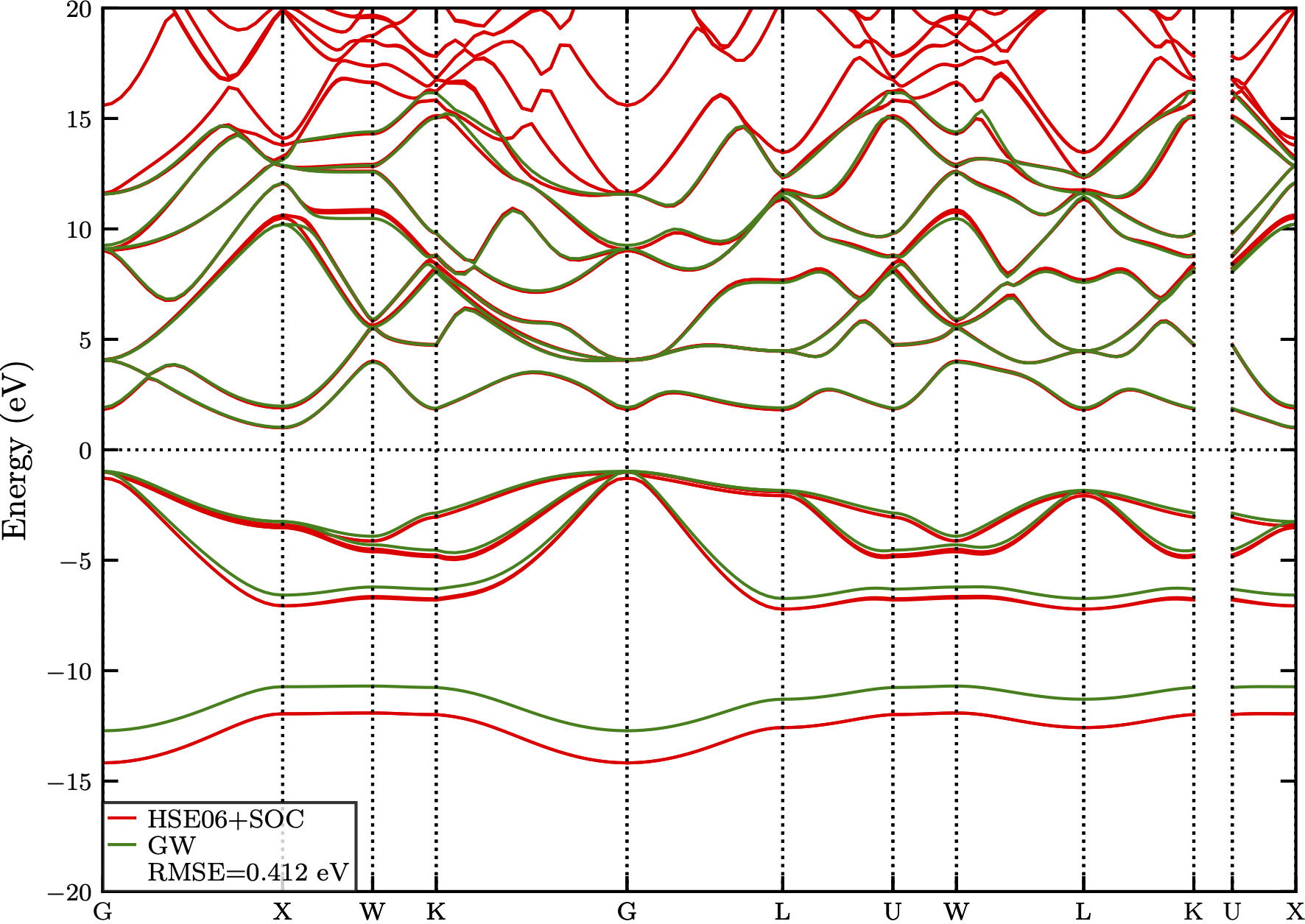Figure 1: The comparison of band structures of AlAs_ZB calculated with GWA and HSE06+SOC. The difference is quantified with a RMSE value of 0.412 eV.

Optionally, if the flag --diffplot is passed to bands_compare.py, the residuals of each matched band for each k-point is plotted as shown in Fig. 2. Each band is assigned a unique color.

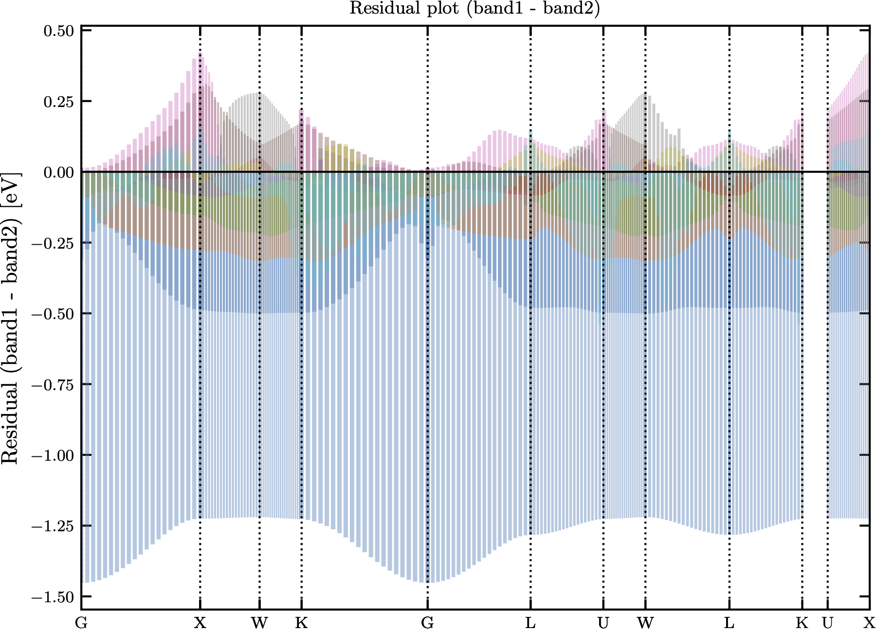Figure 2: The residual plot for comparing AlAs_ZB band structures between GWA and HSE06+SOC.

2. AlAs_ZB GW approximation vs. HSE06 hybrid functional without spin-orbit coupling (SOC)

In Fig. 3, we notice that disabling the spin-orbit coupling in the HSE06 calculation provides a band structure closer to that of the GW approximation. This is mostly emphasized near the HOMO at the $\Gamma$ point where the HSE bands show a slight upward shift.

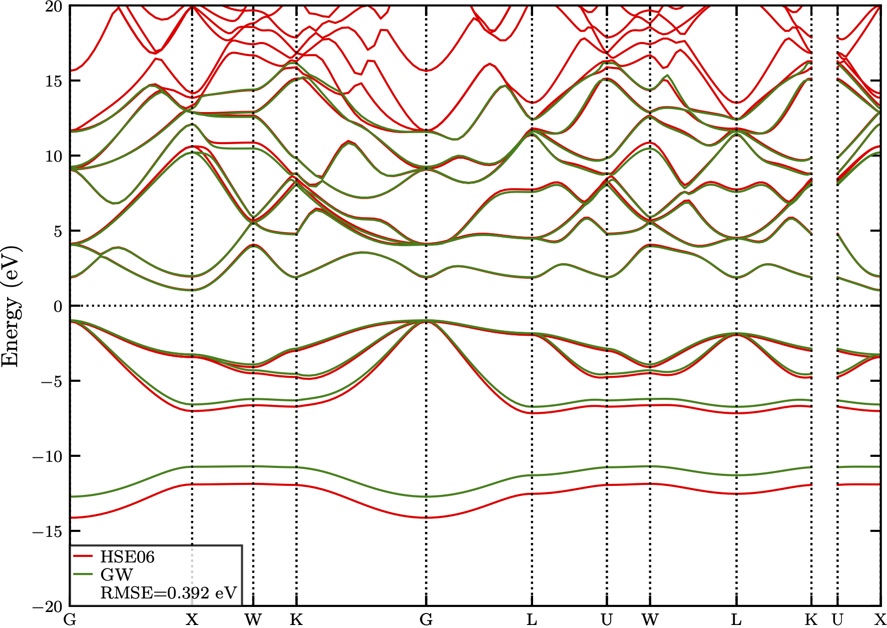Figure 3: The comparison of band structures of AlAs_ZB calculated with GWA and HSE06. The difference is quantified with a RMSE value of 0.392 eV.

3. GaN_ZB with and without auxiliary basis functions

Fig. 4 showcases the differences in the GW band structures of GaN in its Zincblende (ZB) phase calculated with and without auxiliary basis functions. Auxiliary basis functions are additional basis functions to represent the Coulomb operator and help improve the band structure accuracy, especially for materials with higher densities such as MgO (Rocksalt), GaN (Wurtzite) and GaN (Zincblende). As we note in Fig. 4, including an additional auxiliary function to represent a $4f$ orbital to the basis resolves the erroneous band structure of conduction bands obtained from the default calculation. The differences between these two are quantified with a high RMSE value of 1.785 eV.

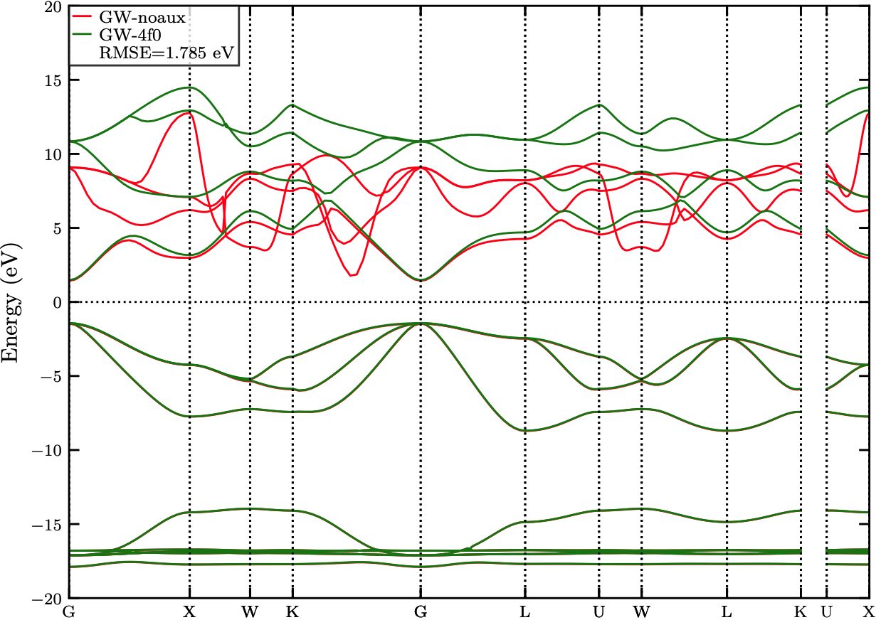Figure 4: The comparison of GW band structures of GaN_ZB calculated with and without 4f0 auxiliary functions. The difference is quantified with a RMSE value of 1.785 eV.

I hope this post helps illustrate the process of computing and interpreting the RMSE for band structure comparisons. Numerical error estimations, alongside visual plots, can provide additional clarity when deciding which settings and parameters provide the best desired outcome for your requirements. Let me know in the comments below if you have any questions or wish to provide any feedback.

References

1. https://www.forbes.com/sites/chadorzel/2016/03/30/why-do-solids-have-band-gaps/ ↩

2. L. Hedin, New method for calculating the one-particle green’s function with application to the electron-gas problem, Phys. Rev.139, A796 (1965). ↩

3. S. Kokott, F. Merz, Y. Yao, C. Carbogno, M. Rossi, V. Havu, M. Rampp, M. Scheffler, and V. Blum, Efficient all-electron hybrid density functionals for atomistic simulations beyond 10 000 atoms, The Journal of Chemical Physics (2024). ↩

4. https://statisticsbyjim.com/regression/root-mean-square-error-rmse/ ↩

5. https://fhi-aims.org ↩

Sign up to get updates on my latest blog posts!

Thank you!

You have successfully joined my subscriber list.